Logistic regression and why it exists

Imagine you’re trying to create a machine learning model to accurately determine if it will rain on a given day. You might try to use a Linear Regression model and plot out a feature like “temperature” for the x-axis and 1 or 0 on the y-axis to represent “RAIN” and “NOT RAIN” respectively. The issue with using a straight Linear Regression model is that the you won’t necessarily get definitive values like 0 and 1. In reality, you probably don’t want a model that’s that confident. Instead, you’d receive values like 0.32, 0.78, 1.4, etc. wherein the model is predicting the likelihood of rain. Higher likelihood equal higher changes of rain. While using a Linear Regression in this context may be effective, it would be much more effective if the model would spit out an actual probability, instead of numbers between 0 and $N$. That’s where Logistic Regression comes in.

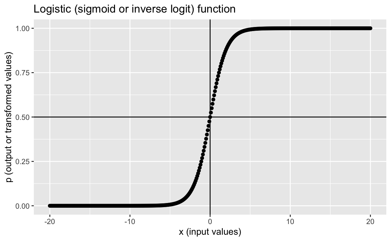
Fundamentally, Logistic Regression takes the output of a linear regression equation and applies a “logistic function” (hence the name Logistic Regression) to it to produce a continuous line between 0 and 1 in the y-axis. This logistic function is also called a Sigmoid Function. The word sigmoid means “s-shaped” and when graphing a sigmoid function it does end up looking like an S-shape.

Logistic Regression has two steps. The first is to get the output from a linear regression equation with as many variables as needed:

Notice that instead of the output being stored in the variable $y’$ that is typical of linear regression in a machine learning context it is stored in the variable $z$. This is because of the second step where we take the output and apply it to the sigmoid function:

The output from this sigmoid function will be between 0 and 1, but will never be exactly 0 or 1. The range of the function is $-\infty < y < \infty$ where both sides of the function are asymptotes.

There are two main applications for Logistic Regression. The first is the one that was mentioned in the introduction of this article: determining a probability. Here, the model’s probabilistic output would be used “as is”; the model’s predicted probability would be the value expected for the intended use case. The second application is to conduct a binary classification. Imagine you’re creating a spam filter and use a Logistic Regression model to determine the probability that a given email is spam. The model would spit out something between 0 or 1, but you have to make a decision with that probability of whether to place it in the user’s inbox or in the spam folder. This would be an instance of binary classification. To learn more about binary classification, read my article here.

The last component of Logistic Regression I’ll touch on is calculating loss. Unlike linear regression that uses either an absolute or squared difference between actual value and predicted value, Logistic Regression requires using a log loss value. Because Linear Regression’s are straight lines, they have a constant rate of changing (slope) making the vertical distance between the actual value and predicted value, squared or not, a fit calculation for loss. However, a logistic function does not have a constant rate of change. Given its s-shape, the function changes much faster in the middle of the function and changes much slower when nearing 0 or 1. Thus, log loss returns the logarithm of the magnitude of the change and not just the distance between actual and predicted values.

where:

• $LL$ = Log Loss
• $(x,y) \in\mathbf{D}$ = dataset containing many labelled examples in the $(x,y)$ pairs
• $y$ = label in labelled example. Since this is logistic regression, every value of $y$ must be either 0 or 1
• $y’$ = model’s prediction (somewhere between 0 and 1), given the set of features in x.

---

Logistic Regression is one of those things that are simple to work through as it’s just one extra calculation on top of a linear model, but offer powerful capabilities to machine learning practitioners. Logistic Regression is one of the core aspects of Neural Networks that allows deep learning models to learn non-linear relationships in data, unlocking many of the applications of machine learning we see today: generative AI, self-driving cars, computer vision, etc. Linear regressions are limited to applications where the data can be represented neatly on a Line of Best Fit. Logistic regressions allow you to go beyond that.